This document demonstrates how to perform clustering in Python using the scikit-learn library. Clustering is an unsupervised learning technique that groups similar data points together based on their inherent characteristics. We will use the adult_income_dataset.csv for this demonstration.
2 Load Data
First, we load the necessary libraries and the income dataset.
Code
import pandas as pdfrom sklearn.cluster import KMeans, AgglomerativeClusteringfrom sklearn.preprocessing import StandardScalerimport matplotlib.pyplot as pltimport seaborn as snsimport scipy.cluster.hierarchy as shcfrom sklearn.decomposition import PCA# Load the income datasetincome_df = pd.read_csv("../data/adult_income_dataset.csv")
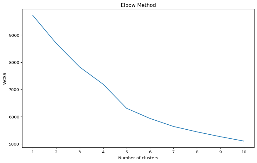
The Elbow Method is a heuristic used to determine the optimal number of clusters in a dataset. We can visualize the total within-cluster sum of squares (WCSS) as a function of the number of clusters.
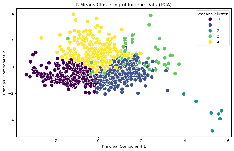
K-Means is a popular clustering algorithm. We will use it to group the income data into clusters. The optimal number of clusters can be determined from the Elbow Method plot.
Code
kmeans = KMeans(n_clusters=5, random_state=42, n_init=10) # Assuming 5 clusters from Elbow Methodincome_df_encoded['kmeans_cluster'] = kmeans.fit_predict(scaled_income)# Visualize the clusters (using first two principal components for visualization)pca = PCA(n_components=2)principal_components = pca.fit_transform(scaled_income)principal_df = pd.DataFrame(data = principal_components, columns = ['principal component 1', 'principal component 2'])principal_df['kmeans_cluster'] = income_df_encoded['kmeans_cluster'].valuesplt.figure(figsize=(10, 6))sns.scatterplot(x='principal component 1', y='principal component 2', hue='kmeans_cluster', data=principal_df, palette='viridis', s=100)plt.title('K-Means Clustering of Income Data (PCA)')plt.xlabel('Principal Component 1')plt.ylabel('Principal Component 2')plt.show()
5 Hierarchical Clustering
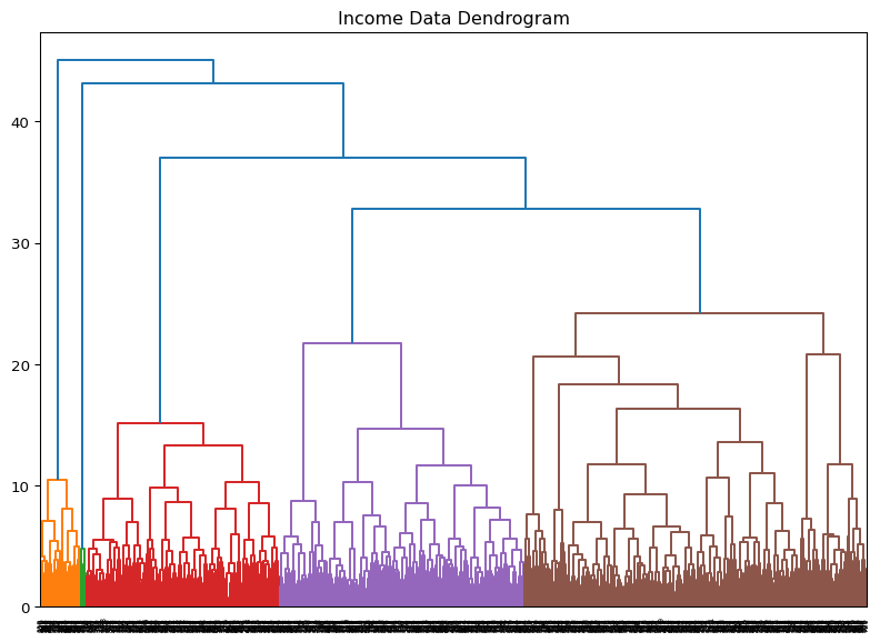
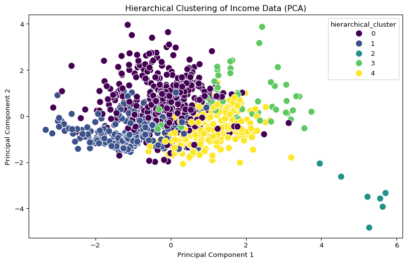
Hierarchical clustering is another common clustering method. We can also visualize the result as a dendrogram.
Code
plt.figure(figsize=(10, 7))plt.title("Income Data Dendrogram")dend = shc.dendrogram(shc.linkage(scaled_income, method='ward'))plt.show()hierarchical = AgglomerativeClustering(n_clusters=5) # Assuming 5 clustersincome_df_encoded['hierarchical_cluster'] = hierarchical.fit_predict(scaled_income)# Visualize the clusters (using first two principal components for visualization)principal_df['hierarchical_cluster'] = income_df_encoded['hierarchical_cluster'].valuesplt.figure(figsize=(10, 6))sns.scatterplot(x='principal component 1', y='principal component 2', hue='hierarchical_cluster', data=principal_df, palette='viridis', s=100)plt.title('Hierarchical Clustering of Income Data (PCA)')plt.xlabel('Principal Component 1')plt.ylabel('Principal Component 2')plt.show()
6 Comparison of K-Means and Hierarchical Clustering
Here’s a comparison of K-Means and Hierarchical Clustering:
Feature
K-Means Clustering
Hierarchical Clustering
Approach
Partitioning (divides data into k clusters)
Agglomerative (bottom-up) or Divisive (top-down)
Number of Clusters
Requires pre-specification (k)
Does not require pre-specification; dendrogram helps
Computational Cost
Faster for large datasets
Slower for large datasets (O(n^3) or O(n^2))
Cluster Shape
Tends to form spherical clusters
Can discover arbitrarily shaped clusters
Sensitivity to Outliers
Sensitive to outliers
Less sensitive to outliers
Interpretability
Easy to interpret
Dendrogram can be complex for large datasets
Reproducibility
Can vary with initial centroids (unless fixed)
Reproducible
7 Conclusion
This document provided a brief overview of clustering in Python using scikit-learn. We demonstrated both K-Means and Hierarchical clustering on the income dataset.
Source Code
---title: "Clustering: Income Data with Python"subtitle: "Using sklearn"execute: warning: false error: falseformat: html: toc: true toc-location: right code-fold: show code-tools: true number-sections: true code-block-bg: true code-block-border-left: "#31BAE9"---## IntroductionThis document demonstrates how to perform clustering in Python using the `scikit-learn` library. Clustering is an unsupervised learning technique that groups similar data points together based on their inherent characteristics. We will use the `adult_income_dataset.csv` for this demonstration.## Load DataFirst, we load the necessary libraries and the income dataset.```{python}#| label: load-data#| echo: trueimport pandas as pdfrom sklearn.cluster import KMeans, AgglomerativeClusteringfrom sklearn.preprocessing import StandardScalerimport matplotlib.pyplot as pltimport seaborn as snsimport scipy.cluster.hierarchy as shcfrom sklearn.decomposition import PCA# Load the income datasetincome_df = pd.read_csv("../data/adult_income_dataset.csv")``````{python}# Handle missing valuesincome_df_clean = income_df.drop('income', axis=1).dropna().sample(n=1000, random_state=42)# Separate numerical and categorical columnsnumerical_cols = income_df_clean.select_dtypes(include=['int64', 'float64']).columnscategorical_cols = income_df_clean.select_dtypes(include=['object']).columns# One-hot encode categorical featuresincome_df_encoded = pd.get_dummies(income_df_clean, columns=categorical_cols, drop_first=True)# Standardize numerical featuresscaler = StandardScaler()income_df_encoded[numerical_cols] = scaler.fit_transform(income_df_encoded[numerical_cols])scaled_income = income_df_encoded.values```## Elbow MethodThe Elbow Method is a heuristic used to determine the optimal number of clusters in a dataset. We can visualize the total within-cluster sum of squares (WCSS) as a function of the number of clusters.```{python}#| label: elbow-method#| echo: truewcss = []for i inrange(1, 11): kmeans = KMeans(n_clusters=i, init='k-means++', max_iter=300, n_init=10, random_state=0) kmeans.fit(scaled_income) wcss.append(kmeans.inertia_)plt.figure(figsize=(10, 6))plt.plot(range(1, 11), wcss)plt.title('Elbow Method')plt.xlabel('Number of clusters')plt.ylabel('WCSS')plt.xticks(range(1, 11))plt.show()```## K-Means ClusteringK-Means is a popular clustering algorithm. We will use it to group the income data into clusters. The optimal number of clusters can be determined from the Elbow Method plot.```{python}#| label: kmeans#| echo: truekmeans = KMeans(n_clusters=5, random_state=42, n_init=10) # Assuming 5 clusters from Elbow Methodincome_df_encoded['kmeans_cluster'] = kmeans.fit_predict(scaled_income)# Visualize the clusters (using first two principal components for visualization)pca = PCA(n_components=2)principal_components = pca.fit_transform(scaled_income)principal_df = pd.DataFrame(data = principal_components, columns = ['principal component 1', 'principal component 2'])principal_df['kmeans_cluster'] = income_df_encoded['kmeans_cluster'].valuesplt.figure(figsize=(10, 6))sns.scatterplot(x='principal component 1', y='principal component 2', hue='kmeans_cluster', data=principal_df, palette='viridis', s=100)plt.title('K-Means Clustering of Income Data (PCA)')plt.xlabel('Principal Component 1')plt.ylabel('Principal Component 2')plt.show()```## Hierarchical ClusteringHierarchical clustering is another common clustering method. We can also visualize the result as a dendrogram.```{python}#| label: hclust#| echo: trueplt.figure(figsize=(10, 7))plt.title("Income Data Dendrogram")dend = shc.dendrogram(shc.linkage(scaled_income, method='ward'))plt.show()hierarchical = AgglomerativeClustering(n_clusters=5) # Assuming 5 clustersincome_df_encoded['hierarchical_cluster'] = hierarchical.fit_predict(scaled_income)# Visualize the clusters (using first two principal components for visualization)principal_df['hierarchical_cluster'] = income_df_encoded['hierarchical_cluster'].valuesplt.figure(figsize=(10, 6))sns.scatterplot(x='principal component 1', y='principal component 2', hue='hierarchical_cluster', data=principal_df, palette='viridis', s=100)plt.title('Hierarchical Clustering of Income Data (PCA)')plt.xlabel('Principal Component 1')plt.ylabel('Principal Component 2')plt.show()```## Comparison of K-Means and Hierarchical ClusteringHere's a comparison of K-Means and Hierarchical Clustering:| Feature | K-Means Clustering | Hierarchical Clustering ||:--------------------|:-------------------------------------------------|:------------------------------------------------------|| **Approach** | Partitioning (divides data into k clusters) | Agglomerative (bottom-up) or Divisive (top-down) || **Number of Clusters** | Requires pre-specification (k) | Does not require pre-specification; dendrogram helps || **Computational Cost** | Faster for large datasets | Slower for large datasets (O(n^3) or O(n^2)) || **Cluster Shape** | Tends to form spherical clusters | Can discover arbitrarily shaped clusters || **Sensitivity to Outliers** | Sensitive to outliers | Less sensitive to outliers || **Interpretability** | Easy to interpret | Dendrogram can be complex for large datasets || **Reproducibility** | Can vary with initial centroids (unless fixed) | Reproducible |## ConclusionThis document provided a brief overview of clustering in Python using `scikit-learn`. We demonstrated both K-Means and Hierarchical clustering on the income dataset.